Diving into the atari-game playing algorithm - Deep Q-Networks
December 01, 2019
Introduction
Reinforcement Learning (RL), the idea of having an agent learn by
directly perceiving its environment and acting to manipulate it, is one
of the great branches of Artificial Intelligence. In this blog post you
will read about a specific breakthrough by DeepMind: its success in
creating a single deep RL architecture that was able to achieve gameplay
in Atari games comparable to that of humans across almost all the
games [1]. They called it DQN, which stands for “Deep
Q-Network”. When its predecessor was first introduced in 2013 [2],
it was, according to the authors, the first system that was able to
learn control policies “directly from high-dimensional sensory input
using reinforcement learning”.
In the coming sections, we will first study Q-learning, a specific RL
algorithm, in its tabular form. Then we will learn how Deep Q-learning
makes it in principle possible to apply RL to more complex problems and
see the so-called deadly triad, which are three properties that are
often present in these problems and lead to divergence. In the section
that follows, we will shortly introduce the two main two tricks that DQN
utilizes for stability, namely experience replay and a fixed target
network. Finally, we answer, through experimentation, how these tricks
can overcome the divergence problems that partly come from the deadly
triad when evaluating the performance in the OpenAI CartPole gym
environment. Concretely, our research questions are:
- Can we find an environment where DQN diverges without the main two tricks employed in that paper, but converges when including the tricks?
- What are the individual contributions that come from using experience replay and a fixed target network?
We will answer these questions by investigating the return, i.e.
cumulative reward, over time achieved by the agent. We expect that
adding both tricks allows the method to converge on the chosen
environment, while only using either of the tricks won’t. Additionally,
we will look at the phenomenon of “soft divergence”, i.e.
unrealistically large Q-values. We hope to shed some light on the
effectiveness of these tricks in less complex environments than Atari
games, allowing beginners in the field of RL to get an intuition of why
DQN works so well, and to think of ways how to improve them even
further.
This post assumes some familiarity with RL. If you feel a lack of prior
knowledge while reading the post, we can recommend reading parts of the
classical introduction into Reinforcement Learning
3 or watching the great (available online)
lecture by David
Silver,
one of the creators of the famous
AlphaZero.
Q-Functions and Q-Learning
In the explanations that follow, there is always the implicit notion of
a Markov-Decision process (MDP): it consists of a finite state space
, a finite action space , a reward space
, a discount factor and transition
dynamics that defines the probabilities to arrive
in the next states with a certain reward, given the current state and
action.
The agent’s goal is to maximize the expected return , which is the
cumulative discounted reward. This can be modeled by -functions,
which represents the expected return for each state action pair
where the rewards are stochastically determined by the actions according
to the agent’s policy (i.e. a distribution over actions
for each state ) and the environment
dynamics . In particular, the -function provides
the information on which action leads to the highest value, given a
state, when following the given behaviour afterwards.
Q-learning is the process of finding the -function of the optimal
policy while following a behaviour policy, e.g. -greedy. This
can be done either in a tabular fashion or using function approximation:
Tabular Q-Learning
In tabular Q-learning, we use the following update rule:
Here, is the next state and is a hyperparameter, namely the learning rate. Under the assumption that each state-action pair is visited infinitely often, this algorithm always converges to the -function of the optimal policy [2].
Note that with growing dimension of the state space the number of possible states grows exponentially. This is also called the curse of dimensionality since it makes tabular -learning and similar tabular methods intractable in high-dimensional spaces. Therefore, we need ways to approximate this process.
Q-Learning with Function Approximation
In order to model these more complex scenarios, we model the Q-function as a parametrised differentiable function that takes in the state and action and, depending on the parameter values, outputs a specific value. In practice, this is often modelled as a function that only takes in the state and outputs a whole array of -values, one for each action. For this blog post, you can assume that is a neural network with as its weights. Then, what is learned are the parameters , of which there are fewer than there are states in the state space. The update rule of semi-gradient Q-learning is then the following:
where is your last state, is the action you chose in that state, is the reward that followed it and is the new state you found yourself in. It is a “semi-gradient method” because Equation (1) is not the full gradient of the loss Instead, the target is treated as a constant.
The Deadly Triad
The resulting method now has the following properties:
- The method is off-policy. That is, no matter what the behaviour policy is, due to the maximization process in the update-rule, we actually directly learn the state-action values of the optimal policy. This allows the agent to explore all possible actions, while at the same time learning what the optimal actions are.
- It is a bootstrapping method. That means, instead of updating its Q-value with an actual outcome of the behaviour, the agent uses an estimate for the update which is itself not perfect and might be biased.
- The method uses function approximation as explained before.
The first two properties were already present in tabular -learning,
but together with the added function approximation it is called the
“deadly triad” since it can lead to divergence of the algorithm1.
In the following section, we explain the tricks that [1]
introduced to tackle the deadly triad and other convergence problems
that may arise in Deep RL. It is largely an open research question how
large the influence of the deadly triad is on divergence problems in
Deep RL, but specifically the fixed target network seems targeted for
precisely that, as described in [4]. Other problems come from the
nature of RL itself, with its highly non-i.i.d. data.
DQN and its Tricks
In principle, the method is just usual semi-gradient -learning with deep neural networks as function approximators. But the authors employ two important tricks:
1. Experience Replay
This describes the process of storing transitions in a memory from which minibatches are later sampled during training.
That process has several advantages:
- It breaks correlations, so that the data is more i.i.d. This reduces variance of the updates and increases stability, since correlated data might lead to too large steps in one direction.
- One has gains in efficiency due to re-used data. Note that -learning is an off-policy method, and so using data from the past, when the behaviour policy was still quite different, does not lead to problems.
2. Fixed Target Network
Recall that the update in semi-gradient Q-learning is given by Equation (1), where is a saved transition and is the current parameter vector.
There can be the following problem with this framework. First, some notation: Denote the target by and imagine it is larger by compared to . Then we obtain and move in the direction of increasing . But is a function approximator, so this is not the only value that changes and similar state-action pairs will change their value as well. Now, and occur only one time-step after and , so they may be perceived as very similar when processed by the -network. Consequently, may increase as much as . The result: may be one larger than again!
I guess you already see the problem: assuming we would run this indefinitely, the Q-value could explode. This happens due to the off-policy nature of the algorithm which does not ensure that gets the relevant feedback later on which would make it smaller again.
For this problem, it may help to fix the target network, which was proposed in [1] for the first time. In that framework, you have parameters which you update constantly, and parameters which you hold constant for timesteps, until you update them to and hold them constant again. This is claimed to prevent the spiraling that we describe here.
The Experiment
Aim of the Experiments
The experiments we run aim to visualize the impact that the tricks of DQN have. Note that in [1], the authors find that each of the two tricks, experience replay and a fixed target network, have their own contribution to the success of the agent and that their contribution amplifies when they are combined. We are interested in whether we can confirm these results in a simpler environment and highlighting the individual contributions of the effects.
The self-written source code of the experiments can be found on GitHub2, where we reference to others if we were inspired by their work.
The Environment
The desiderata for our environment were the following:
- It is simple enough to allow easy experimentation.
- It is complex and difficult enough so that DQN without experience replay and a fixed target network is not able to solve it.
With these criteria in mind, we will see if the tricks proposed in DQN make it solvable.
We qualitatively reviewed the performance of our model trained on all classic control environments of OpenAI Gym3. Performance is measured as the (negative) episode duration (sign dependant on the whether the agent is tasked to have long or short episodes), and plotted over the training period. We found that the Acrobot-v1 and MountainCar-v0 environments would require further modifications to DQN to be solvable, i.e. even the tricks were not able to lead to convergence. However, the Cartpole-v1 environment displayed exactly the required properties: it diverged when using standard semi-gradient Q-learning with function approximation, but converged when adding experience replay and a target network. In this environment the return is the total number of steps that the pole stays upright, with the upper limit of the number of episodes being 500.
Methods
We have trained the network in the following four versions:
- vanilla semi-gradient Q-learning with function approximation.
- the same as (1) and including experience replay.
- the same as (1) and including a fixed target network which is updated every steps. We experiment with different values of in the set .
- a combination of (2) and (3). This is the full training process proposed in [1].
Each variant uses the same simple neural network implemented in PyTorch:
class QNetwork(nn.Module):

    def __init__(self, num_s, num_a, num_hidden=128):
        nn.Module.__init__(self)
        self.l1 = nn.Linear(num_s, num_hidden)
        self.l2 = nn.Linear(num_hidden, num_a)

    def forward(self, x):
        x = F.relu(self.l1(x))
        x = self.l2(x)
        return x
All variants use the same static set of hyperparameters listed in the table below, where we also explain the reasoning behind their choice.
| Hyperparameter | Value | Rationale |
|---|---|---|
| Number of episodes | Methods that proved convergence properties converge after around 50 episodes. | |
| Batch size | Standard ”exponent of 2” value with no particular meaning. | |
| Discount Factor | Hand-picked during experimentation and implementation process. | |
| Learning Rate | Hand-picked during experimentation and implementation process. | |
| Memory Capacity | Hand-picked during experimentation and implementation process | |
| Replay Start Size | Batch Size | After state transitions, we begin training, since then the memory contains enough transitions to fill a batch. |
| Seed | Set of different seeds used to ensure reproducibility and to get uncorrelated results. | |
| 1 | At the beginning we play a maximal exploration strategy since the policy did not find good behaviour yet. | |
| We don’t act greedily even during validation, so that the agent cannot overfit on the training experience | ||
| Within updates, is linearly annealed to . Hand picked during implementation as it gave fast convergence. | ||
| Optimizer | ADAM (default parameters) | State of the art optimizer suitable for most applications. |
| NN architecture | Input dim: number of states, i.e. 4; Hidden dim: 128 followed by ReLU; Output dim: number of actions, i.e. 2 | Hand-picked based on problem and input complexity. |
The Implementation
We have utilized the code obtained during Lab sessions of the course Reinforcement Learning at University of Amsterdam as the skeleton of our code, and added a flag to enable/disable the experience replay trick, and added an integer input to define for how many steps the target network would be fixed (1 meaning it is updated each time i.e. it is not fixed). All the environments used are from the OpenAI Gym library. For the implementation we use several open-source standard machine learning python packages (for details see the source code). The experiments are run on a regular laptop with Intel i5-7200U CPU and 8GB of RAM on which a single run of 100 episodes takes about 30 seconds. This means that the results we obtained here can easily be checked on your computer in a few minutes.
Results
For assessing the performance of our agent, we look both at the return and at so-called soft divergence. Note that with return, we always mean the undiscounted return, even if the agent discounts, as in our case, with . That is, we treat not as part of the objective, but as a hyperparameter. We will explain soft divergence in the corresponding subsection.
Return
We will present the results of the experiments with plots in which the x-axis represents the number of the episodes and the y-axis represents the return obtained during validation. This means that every 5 episodes we take the trained model, fix to 0.05 and evaluate the performance of this model, without training it during this process.
Each curve belongs to one variant of the algorithm. For each variant, we train the agent from scratch 10 times with different seeds and create the line by averaging the returns. The shaded area around each curve is the confidence interval (i.e. it represents ).
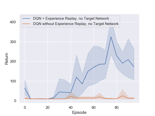
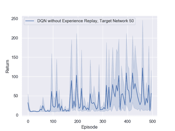
Figure 1 presents the comparison between the models with and without experience replay. In both cases, we did not use the fixed target network. The picture clearly displays the difference in quality of the two different methods showing that experience replay is a very important factor of convergence in this environment. We also ran the method without experience replay for 500 episodes, but still did not see any clearly improving values as seen in Figure 6 in the appendix.
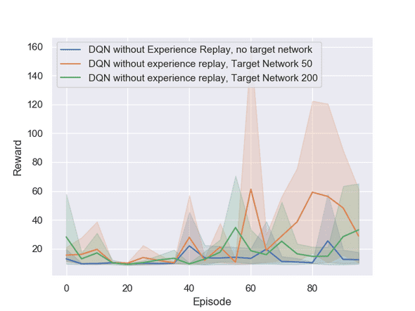
In Figure 2 we display the effect of the target network with different update rates on the obtained returns while turning experience replay off. We observe that the version with an update rate of is often in the lead, however, we do not see an obvious statistical effect of the target network alone. To keep the graphs uncluttered, we do not show the values of 100 and 500 which perform roughly equal to the 50 value.
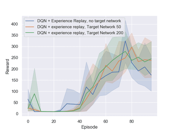
In Figure 3 we illustrate the effect of the combination of both tricks. In the case with experience replay, over large parts of the training process the version with an update rate of steps is leading, although there can not be any statistical significance inferred in comparison to the update rate of and (no target network).
Finally, in Figures 1 and [3], we observe that the average episode duration decreases after 75 episodes. To investigate if this is a systematic or purely random effect, we trained the model for 300 episodes which can be seen in Figure 7 in the appendix. In both settings the performance seems to decrease slightly after 100 episodes. To be on the safe side, we therefore suggest to periodically take snapshots of the weights and in the end use the model with the highest average episode duration.
Soft Divergence
Now we look at assessing the so-called soft divergence. Soft divergence was for the first time studied in 4 as follows:
Let be our discount rate, in our case . Since our rewards are all in the interval (actually, it is always until the agent loses or the episode is over), there is a bound on the maximally achievable true Q-values. We can see this by bounding the discounted return:
In our case, this bound is . Now, soft divergence is the phenomenon of learned Q-values that exceed this bound. This is connected to the deadly triad: off-policy learning with bootstrapping and function approximation can lead to a situation in which the Q-values chase the targets, which themselves can get bigger and bigger until they exceed realistic bounds.
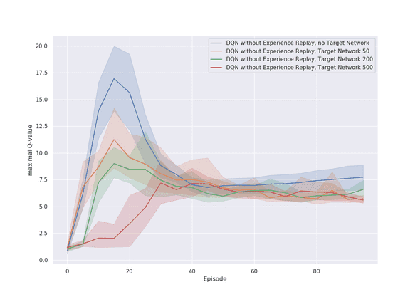
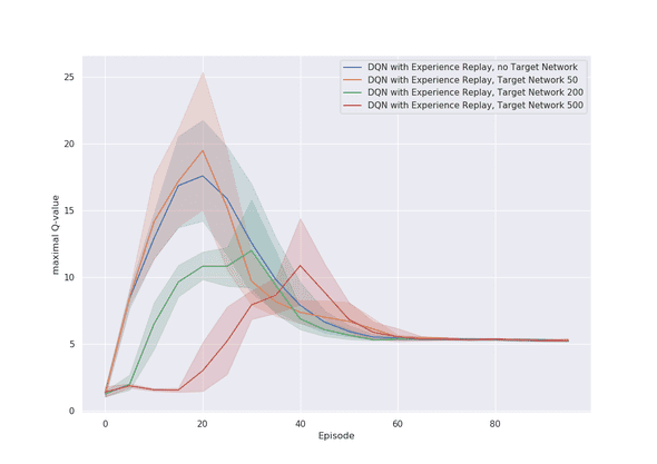
In order to assess the presence of soft divergence, we measure the maximal Q-values that appear within evaluation episodes. In Figure 4, you can find this for the case without experience replay, and in Figure 5 for the case with experience replay.
First of all, we can see that if we use experience replay, the maximal Q-value converges precisely to . This is expected, since we already know that an agent using experience replay achieves high return, and so if the Q-value measures the return correctly, it should output something close to the optimal value, which is .
However, the version without experience replay actually shows soft divergence, with Q-values being consistently too large in the end of training with values ranging between and . Additionally, since we already know that the agent performs very bad, we would actually expect Q-values lower than . Now we get an explanation for why the agent is not able to perform properly: the measurements of the Q-values are partly too high during the entire training process, and therefore not accurate, and cannot guide the agent to the actions with the best behaviour.
Another interesting phenomenon can be observed by looking at the differences between the different target network update rates. In both plots we see that, in the beginning of the training process, the Q-values get considerably larger than , ranging up to . That is, all versions of the algorithm show soft divergence in the first 50 episodes, with a peak after episodes. One explanation might be the maximization bias which is present in Q-learning. Maximization bias is a phenomenon which happens when the algorithm overestimates the Q-values as a consequence of the arguments in the update rule. In practice, this bias has been studied and can be solved for example with double Q-learning explained in [5]. However, since we did not include experiments using double Q-learning, we cannot assess the validity of this explanation.
A second and complementary explanation for this might be the following: in the beginning of training, the learned representations of the Q-network are very bad and might not be successful in distinguishing between different state-action pairs. If that happens, then the increase of one Q-value might just increase the Q-values of all other states in the same way, which creates the already explained phenomenon that Q-values can become unbounded. This would also explain why the problem is less severe when using the fixed target network, and even less severe if the updates of the parameters happen less often.
Conclusion
In this blog post we have analyzed what effect the tricks experience replay and a fixed target network have on the convergence of the DQN algorithm. Our experiments have shown that, by itself, the DQN algorithm without experience replay and fixed target network fails to converge.
Furthermore, we observe that experience replay has a significant impact on the objective, i.e. return, whereas the fixed target network showed almost no effect on that. This is different from what we expected, as we initially expected that only the addition of both tricks would allow the agent to perform optimally.
For the large effect of the experience replay on the return, we believe this is because in a physical system like the cart pole environment subsequent state observations are deterministically dependent. This is the strongest form of correlation and might lead to too large steps in one direction. This can be specifically crucial, because a fast move in one direction of the cart can lead to a change of orientation of the pole in the other direction and to the end of the episode.
The small effect of the fixed target network on the return is contradicted, however, by analyzing its effect on soft divergence. We saw that the fixed target network actually plays an essential role in mitigating the initially very high Q-values seen in all variants of the algorithm. This does not itself change the return of the agent after convergence, since in all cases, the algorithm is able to correct for the mistake of vastly too large initial Q-values. Still, these results hint that in more complex environments, we would also see an influence of the fixed target network on the return achieved by agents as updating the target network more rarely can help fight the soft divergence.\
We conclude that generally DQN contains strong and theoretically sound ideas, and we saw that both tricks can, in different ways, help avoiding divergence. However, to train it successfully and to use the utility of the tricks fruitfully, still requires practice and effortful tuning.
Appendix
DQN without Experience Replay after 500 Episodes
DQN with Experience Replay after 300 Episodes

Referenes
[1] Human-level control through deep reinforcement learning
[2] Playing Atari with Deep Reinforcement Learning]
[3] Sutton & Barto: Reinforcement Learning Book
[4] Deep Reinforcement Learning and the Deadly Triad
[5] Double Q-learning
-
It is out of the scope of this blog post to go into the details as to why the deadly triad can lead to divergence. We recommend the interested reader to read chapter of [@sutton2018reinforcement].
↩ -
https://github.com/YoniSchirris/rl-lab3
↩ - ↩